In this blog post, we’ll delve into the fascinating world of 3D point cloud data analysis using Python. Point cloud data is a collection of 3D points in space, often captured using techniques like LiDAR or RGB-D cameras. We’ll explore how to generate synthetic clusters of 3D points, perform DBSCAN clustering, and visualize the results using libraries like NumPy, Matplotlib, and Open3D.
Overall, python is a very valuable programming language for point cloud analysis. Its simplicity and versatility make it an ideal choice for processing and analyzing complex 3D data. By leveraging Python’s rich ecosystem of libraries and tools, such as NumPy, Matplotlib, and Open3D, researchers and engineers can effortlessly manipulate, visualize, and gain insights from point cloud data. Whether it’s for robotics, autonomous vehicles, or virtual reality applications, Python’s ease of use empowers professionals to unlock the potential of 3D data without the steep learning curve associated with other languages.
In this post, we will identify clusters in our point cloud as an example of point cloud processing. However, this is only one of many possibilities offered by Python and its frameworks such as Open3d or scikit-learn. Clustering is a fundamental technique in data analysis that plays a critical role in the point cloud space. The inherent complexity of 3D data requires intelligent organization, and this is where techniques like DBSCAN shine. Density-Based Spatial Clustering of Applications with Noise (DBSCAN) is unique in its ability to uncover clusters of varying shapes and sizes within point clouds. By automatically identifying dense regions while excluding noisy data points, DBSCAN streamlines the exploration of 3D structures and patterns. This critical process not only enhances understanding, but also paves the way for more informed decision-making in fields ranging from environmental modeling to architectural design.
So let’s get started.
Setting Up the Environment
Before we dive into the code, let’s ensure we have the necessary libraries installed. We’ll be using NumPy for numerical operations, Matplotlib for visualization, and Open3D for handling 3D data. To get started, make sure to have Open3D installed using the following command:
pip install open3dAnd we import the necessary packages:
import numpy as np
import matplotlib.pyplot as plt
from mpl_toolkits.mplot3d import Axes3D
import open3d as o3d
Generating Synthetic Clusters
To begin our exploration, let’s generate synthetic clusters of 3D points. We’ll define cluster parameters including means and covariances for each cluster. These parameters will help us generate random points around these clusters.
np.random.seed(1)
num_points = 300
cluster_params = [
 {"mean": np.array([0, 0, 0]), "cov": np.array([[1, 0.5, 0.5], [0.5, 1, 0.5], [0.5, 0.5, 1]])},
 {"mean": np.array([4, 4, 4]), "cov": np.array([[1, -0.8, -0.8], [-0.8, 1, -0.8], [-0.8, -0.8, 1]])},
 {"mean": np.array([-3, -4, -5]), "cov": np.array([[1, -0.8, -0.8], [-0.8, 1, -0.8], [-0.8, -0.8, 1]])}
]

clusters = []
for param in cluster_params:
 cluster = np.random.multivariate_normal(param["mean"], param["cov"], num_points // 3)
 clusters.append(cluster)
points = np.vstack(clusters)
Visualizing the Synthetic Point Cloud
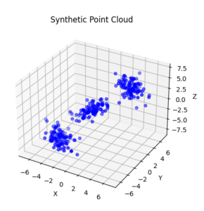
With our synthetic points generated, it’s time to visualize them in a 3D plot using Matplotlib. We’ll create a scatter plot of the points, setting their coordinates as the x, y, and z values
fig = plt.figure()
ax = fig.add_subplot(111, projection='3d')
ax.scatter(points[:, 0], points[:, 1], points[:, 2], c='b', marker='o')
ax.set_xlabel('X')
ax.set_ylabel('Y')
ax.set_zlabel('Z')
ax.set_title('Synthetic Point Cloud')
plt.show()
Resulting in the following output
Clustering with DBSCAN
Now, we’ll perform clustering on our point cloud using the Density-Based Spatial Clustering of Applications with Noise (DBSCAN) algorithm. DBSCAN is well-suited for data like point clouds, where clusters might have varying shapes and densities.
point_cloud = o3d.geometry.PointCloud()
point_cloud.points = o3d.utility.Vector3dVector(points)
eps = 1.2 # Distance threshold for points in a cluster
min_points = 10 # Minimum number of points per cluster
dbscan_labels = np.array(point_cloud.cluster_dbscan(eps=eps, min_points=min_points, print_progress=True))

print("Cluster labels (with -1 indicating noise): ")
print(f"Labels: {dbscan_labels}")
Visualizing the Clustering Results
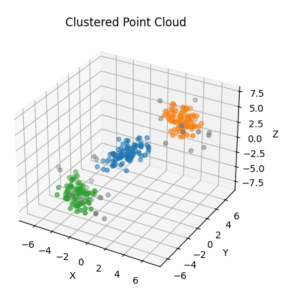
To better understand the clustering results, we’ll visualize them by coloring the points based on their cluster labels. Points assigned to the same cluster will have the same color, and noise points will be colored in gray
colors = plt.get_cmap("tab10")(dbscan_labels)
colors[dbscan_labels == -1] = [0.5, 0.5, 0.5, 1]
fig = plt.figure()
ax = fig.add_subplot(111, projection='3d')
ax.scatter(points[:, 0], points[:, 1], points[:, 2], c=colors)
ax.set_xlabel('X')
ax.set_ylabel('Y')
ax.set_zlabel('Z')
plt.show()
As we can see in the following image we found three clusters and few points that are considered noise under our parameter configuration.
Conclusion
In this tutorial, we’ve started our journey in the realm of 3D point cloud data analysis. We’ve generated synthetic clusters, utilized the DBSCAN algorithm for clustering, and visualized the results in an a 3D scatter plot. This is just a glimpse into the potential of working with 3D data in Python. As technology continues to advance, mastering these techniques will undoubtedly unlock new opportunities for innovation in various fields, from robotics to augmented reality.